Apologies for the embarrassingly bad pun in the title.
Distributions in general
First, it’s necessary to talk about distributions on an arbitrary open set 


Anyway, the idea here will be to consider auxiliary spaces 


Now, any functional 


As before, we can multiply a distribution by a function, and we can differentiate a distribution. We can also talk about convolutions of a distribution with a compactly supported distribution or with afunction, and these satisfy all the usual identities. (I’m not inclined to write out all the details, though.) So it is still interesting to talk about fundamental solutions to PDE which may not be tempered.
Malgrange-Ehrenpreis
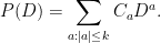
So, let’s fix a constant-coefficient differential operator
The big theorem here is:
Theorem 1 (Malgrange-Ehrenpreis)
There is a distributionwith
i.e. a fundamental solution.

The precise statement is proved in the book by Hormander (Linear Partial Differential Operators), where he proves in fact that the fundamental solution belongs locally to a generalization of the Sobolev spaces that we shall meet presently. However, I’m not inclined to write out all the details right now, so I’ll prove the following weaker statement:
Theorem 2 Given
.
Note that since convolution still works with arbitrary distributions and compactly supported functions, we get the previous theorem about local solvability of 

This is the key lemma:
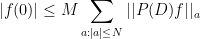
Lemma 3
Let. Then there exist
such that
forand the seminorms defined as before.
What does this mean? The map 


Polynomials
To get the estimates, we will use

together with 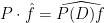

Lemma 4
Letbe analytic in a neighborhood of the closed unit disk, and
. Then

This looks a lot like Cauchy’s formula, and indeed it reduces to that if we replace the polynomial 


However, we have the problem that polynomials in general have roots, which will cause some problems in our estimates. All the same, if
is bounded below and polynomially at 
Lemma 5
Letsuch that for any
, we have

We can of course assume that we have an expression 


we will be done. This follows from observing that we may consider the pair

If we now apply the previous lemma to this pair, we find the claim.
Next time, we’re going to use these lemmas to get the appropriate bounds necessary to prove Theorem 2.

January 26, 2013 at 6:02 am
why do we need to consider partial differential operator?what is it’s applications
January 26, 2013 at 6:45 am
That’s a broad question. I don’t think I could do better than pointing you to the wikipedia page, and mentioning that many physical phenomena are described by PDEs.