I’ve set a tentative goal of heading towards the solution of the Dirichlet problem on compact manifoldw-with-boundary and Hodge theory; these will require various preliminaries, since of course it will be more fun to do it this way than to restrict to open sets in  . Today I will go through some of the basics of how the well-known operators from multivariable calculus work more generally on a Riemannian manifold, which will be necessary in the sequel. (I shamelessly took the title of the post from a book I haven’t read.)
Recall the well-known operator on functions of  -variables, the Laplacian

The problem is,  doesn’t transform nicely with respect to changes in coordinates, and since we want to define the Laplacian on manifolds, this causes a problem. However, it can be done on a Riemannian manifold. The idea is to use the formula

which is immediate from the definitions on  . The key point is that
  and
and  make sense on any Riemannian manifold—from, respectively, vector fields to functions and from functions to vector fields.
Grad
Let’s start with . The basic property of  for
for  a smooth function on is that for any vector
  ,
,

So, we can use the formula  to define as a vector field on any Riemannian manifold, where the inner product is now with respect to the Riemannian metric. If we consider the unit vector in the direction as , the directional derivative of a function is always 1, same as before. Of course, to be meaningful the function must have a noncritical point there.
Div
That’s one. is a little tricker. First, recall that we have a volume element  , and that on has the property that

This is nontrivial. First, recall that the Lie derivative has a derivation-like property with respect to the wedge product (basically, the product rule), so

Now

(To see this, apply both sides to  , and use the way
  deals with the pairing between tangent and cotangent vectors. Cf. the first few chapters of any introductory book on differential geometry.) It follows by antisymmetry that (*) holds. This uniquely determines
  since the vector bundle of -forms is a line bundle. Now I claim that all this makes perfect sense on any Riemannian manifold if
  is a vector field. All we have to do is construct the -form.
The volume form
The idea is to choose an orthonormal moving frame  for the cotangent space, and let

A few words are to be said here. That are orthonormal means with respect to the induced inner product on the cotangent spaces coming from the isomorphism between them and the tangent spaces from the inner product. Next, it is clear by definition of a vector bundle that we can always locally choose a moving frame (i.e., sections over an open set which form a basis for the cotangent space at each point), but to get orthonormality, we have to use the Gram-Schmidt process. Anyway, it is clear that this definition includes the volume form on , but perhaps it is unclear whether this is really well-defined. In fact, it isn’t unless we choose an orientation on  (if possible). So, let’s revise our definition.
  is defined as above precisely when is an oriented orthonormal basis. So has the unique property that for any oriented orthonormal basis
  for
for  , we have
(It is clear that this is true when  is the dual
  to
to  , and the general case follows because the change from to a general oriented orthonormal is made by making an orthogonal transformation whose determinant must be
  (not
(not  ) because of the orientation hypothesis. This shows additionally that we’ve defined something uniquely.)
So, on an oriented Riemannian manifold, we can define via
as before. If we don’t have an orientation globally, we can choose one locally and still define this way; notice that changing the orientation flips but does not alter . So in the long run, the orientation becomes irrelevant.
The trace of the covariant derivative
There is another way of defining that is also of interest. Given , we can define the covariant derivative  as the (1,1) tensor
Of course,  comes from the Levi-Civita connection. Then I claim:

In other words, if  is an orthonormal basis for the tangent space at a point, we have
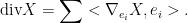
(Note that I use subscripts for tangent vectors, superscripts for cotangent vectors. This should minimize notational confusion.) Because of the derivation-like property of  (i.e.
(i.e.  ), it follows that

which would not be so easy to prove from the Lie derivative definition. (To see the identity, choose the such that one is in the direction of , and the others orthogonal to it.)
Note that the boxed statement is an obvious fact in if we choose the as  .
.
To prove the boxed statement, we will use the fact that the volume form is parallel. This is simply because parallelism preserves the property of being an orthonormal basis, and orientation must be preserved as well (by continuity). In particular, if we choose an orthnormal frame of cotangent vectors , it follows that
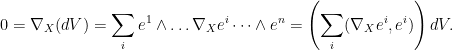
So

which equals by necessity

Here of course the inner product is the inner product on the cotangent space. Let be the dual basis to ; this is an orthonormal frame on some neighborhood (so they are vector fields, not just tangent vectors). Then the quantity in parenthesis, which is , equals

by the way the covariant and Lie derivatives interact with the pairing between tangent and cotangent spaces; this becomes
![\displaystyle \sum_i \left< \nabla_X e_i -[ X, e_i] , e_i \right> = \sum_i \left< \nabla_{e_i} X , e_i \right>](https://s0.wp.com/latex.php?latex=%5Cdisplaystyle+%5Csum_i+%5Cleft%3C+%5Cnabla_X+e_i+-%5B+X%2C+e_i%5D+%2C+e_i+%5Cright%3E+%3D+%5Csum_i+%5Cleft%3C+%5Cnabla_%7Be_i%7D+X+%2C+e_i+%5Cright%3E+&bg=ffffff&fg=000000&s=0&c=20201002)
by symmetry of the Levi-Civita connection.
Next, I’ll talk about how the divergence theorem can be generalized to Riemannian manifolds.

January 12, 2010 at 1:34 pm
Aha, you can follow my post at http://anhngq.wordpress.com/2009/12/05/r-g-laplace-beltrami-operator/ where I did construct the following
in very details.