Tempered distributions

The next basic tool we’re going to need is the theory of distributions.

Distributions

Distributions are extremely useful because they are both fairly general (including both all integrable functions and things like the Dirac delta function) but also allow for operations such as differentiation. So oftentimes we can obtain distribution solutions to differential equations we are interested in.

Actually, we’ll only discuss here tempered distributions. A tempered distribution is a linear functional ${\phi: \mathcal{S} \rightarrow \mathbb{C}}$ . Clearly the tempered distributions form a vector space ${\mathcal{S}'}$ ; it is a locally convex space if we endow it with the weak* topology. It must now be seen how distributions generalize functions. So, if ${f \in L^p(\mathbb{R}^n)}$ for any ${p, 1 \leq p \leq \infty}$ , then ${f}$ can be made into a distribution

$\displaystyle w \rightarrow \int_{\mathbb{R}^n} wf dx, \ w \in \mathcal{S}.$

In fact, we could just assume that ${f}$ grows polynomially. In particular, we have an imbedding ${\mathcal{S} \rightarrow S'}$ .

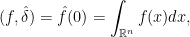
An example of a distribution that is not a function is the Dirac distribution ${\delta}$ mapping ${f \rightarrow f(0)}$ .

Operations on distributions

We use ${(\cdot, \cdot)}$ to denote the bilinear pairing ${\mathcal{S} \times \mathcal{S}' \rightarrow \mathbb{C}}$ . By abuse of notation, when ${f,g \in \mathcal{S}}$ , we will write ${(f,g) := \int f(x) g(x) dx}$ as well; this fits with the imbedding of ${\mathcal{S}}$ into ${\mathcal{S}'}$ .

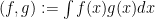
Using this form, we can extend many of the normal operators on ${\mathcal{S}}$ (whose elements are extremely well-behaved) to ${\mathcal{S}'}$ . Let ${T: \mathcal{S} \rightarrow \mathcal{S}}$ be a continuous map; suppose it has an adjoint map ${T': \mathcal{S} \rightarrow \mathcal{S}}$ , i.e.

$\displaystyle (f,Tg) = (T'f, g), \ f,g \in \mathcal{S}.$

Then for ${\phi \in \mathcal{S}'}$ , we can define ${T\phi \in \mathcal{S}'}$ by the same formula

$\displaystyle (f, T\phi) := (T'f, \phi).$

Since ${T'}$ is continuous on ${\mathcal{S}}$ , it is also continuous on ${\mathcal{S}'}$ in the weak* topology, as is easily checked.

The basic example of this is a differential operator. Writing ${D_j:=\frac{\partial}{\partial x_j}}$ , we see the identity

$\displaystyle (D_j f,g) = \int_{\mathbb{R}^n} D_j f(x) g(x) dx = - \int_{\mathbb{R}^n} f(x) D_j g(x) dx = -(f, D_jg)$

for ${f,g \in \mathcal{S}}$ is immediate from integration by parts. So given a distribution ${\phi}$ , we may define ${D_j \phi}$ by ${(f,D_j \phi) = -(D_j f, \phi)}$ . So any multi-index ${a \in (\mathbb{Z}_{\geq 0})^n}$ induces an operator ${D^a }$ on ${\mathcal{S}'}$ . As a result, we can talk about distribution solutions to differential equations, which will become important in the future.

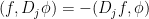
For example, it is heuristically said that, on ${\mathbb{R}^1}$ , the Heaviside function ${H}$ defined by ${H(x) = 0}$ for ${x \leq 0}$ , ${H(x)=1}$ for ${x>0}$ is the antiderivative of the delta function. This is actually true in the sense of distributions:

$\displaystyle \int_{\mathbb{R}} f'(x) H(x) dx = -f(0), \ f \in \mathcal{S}(\mathbb{R}).$

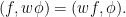
The next basic example of an operation on a distribution is multiplication by a function. Clearly if ${w \in S}$ the map ${\mathcal{S} \rightarrow \mathcal{S}}$ , ${f \rightarrow wf}$ , is self-adjoint, so we define ${w\phi}$ for a distribution ${\phi}$ by

$\displaystyle (f, w\phi) = (wf, \phi).$

Fourier transforms and convolution

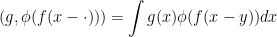
We can also do convolution—i.e., we can convolve a distribution ${\phi}$ with an element ${f}$ of ${\mathcal{S}}$ . I claim that this is actually the function ${(\phi \ast f)(x) := \phi( f(x-\cdot))}$ . Indeed, where ${\phi}$ denotes the application to a function of ${y}$ ,

$\displaystyle (g, \phi(f(x - \cdot))) = \int g(x) \phi( f(x - y)) dx$

which becomes

$\displaystyle \int \phi\left(g(x) f(x - y) \right) dx = \phi\left( \int g(x) f(x-y) dx \right) = \phi(g \ast f)$

since the partial sums of the integral defining ${g \ast f}$ converge in ${\mathcal{S}}$ to ${g \ast f}$ . Note that the function ${\phi \ast f}$ increases at most polynomially at ${\infty}$ .

The final example we are interested in today is the Fourier transform of a distribution. This is now routine though, in view of the adjoint property proved the previous time; we just have to define ${\hat{\phi}}$ via

$\displaystyle (f, \hat{\phi}) = ( \hat{f}, \phi).$

(The reversal from ${\tilde{f}}$ to ${\hat{f}}$ is because the bilinear form we’ve defined is complex-linear; it’s not the hermitian inner product on ${L^2}$ , so there’s a bit of a change.)