Symplectic manifolds, time-dependent vector fields, and Cartan’s magic formula

The purpose of this post is to discuss a few basic facts about differentiable manifolds and state the Darboux theorem, which I will prove next time. (People who are looking for a more ambitious leap into symplectic geometry might want to try lewallen’s two posts over at Concrete Nonsense.)

A symplectic manifold is a smooth manifold ${M}$ equipped with a closed symplectic 2-form ${\omega}$ . In other words, ${\omega}$ is alternating and nondegenerate on each tangent space ${T_p(M)}$ .

The basic example of a symplectic form is

$\displaystyle \sum_i dx^i \wedge d\xi^i$

on ${\mathbb{R}^{2n}}$ with coordinates ${x^i, \xi^i, 1 \leq i \leq n}$ .

This can also be written in a more invariant form, which will also give an invariant manner of making the cotangent bundle ${T^*M}$ of any manifold ${M}$ into a symplectic manifold. First, we define a 1-form ${\alpha}$ on ${T^*M}$ . Let ${p: T^*M \rightarrow M}$ be the projection downwards. Given ${v \in T^*M}$ lying above ${\xi \in T^*M}$ , define

$\displaystyle \alpha(v) = \xi( p_*(v)).$

To make this clearer, here is an interpretation in local coordinates. Let ${x^1, \dots, x^n}$ be local coordinates for ${M}$ . Then ${x^1, \dots, x^n, \xi^1, \dots, \xi^n}$ coordinates for ${T^*M}$ . Then

$\displaystyle \alpha = \sum \xi^i dx^i$

as is easily checked by working through the definitions. So we can define a canonical 2-form ${\omega}$ as ${\omega = - d \alpha}$ ; this makes ${T^*M}$ into a symplectic manifold.

The Darboux theorem

Unlike the case for Riemannian manifolds, symplectic manifolds are always locally isomorphic—or more precisely, symplectomorphic, i.e. diffeomorphic in a manner preserving the symplectic forms. There is thus no analog of the Riemann curvature tensor for symplectic manifolds.

The proof will rely on the Moser trick, which constructs the diffeomorphism using an isotopy induced by a certain time-dependent vector field.

Theorem 1 Let ${(M,\omega)}$ be a symplectic manifold. If ${p \in M}$ , then there is a neighborhood ${U \subset M}$ containing ${p}$ and a diffeomorphism ${f: V \rightarrow U}$ for ${V \subset \mathbb{R}^{2n}}$ such that ${f^*\omega = \omega_0}$ , where ${\omega_0}$ is the canonical 2-form.

Lie derivatives and Cartan’s magic formula

Recall the operation of Lie derivative. Given a vector field ${X}$ on a manifold ${M}$ generating a local flow ${\phi}$ and a tensor ${T}$ , define

$\displaystyle L_X(T)(p) := \lim_{t \rightarrow 0} \frac{ \phi_t^*(T)(p) - T(p)}{t}.$

This is easily seen to be a derivation operator, i.e.

$\displaystyle L_X(T \otimes U) = L_X(T) \otimes U + T \otimes L_X(U)$

and one that commutes with contractions. It also commutes with symmetrization and alternation, so preserves forms.

Proposition 2 On vector fields ${T}$ , the Lie derivative is just the Lie bracket: ${L_X(T) = [X,T]}$ .

This is proved by some fairly involved means in Spivak or Kobayashi-Nomizu. I don’t know why they don’t use the following argument, which I learned from Volume one of Partial Diffential Equations by Michael Taylor.

The idea is that since this is an invariant assertion, we can choose the local coordinates wisely. For instance, let’s suppose that we want to establish this at ${p \in M}$ , and ${T(p) \neq 0}$ . Then (using the flow ${\phi}$ —this is a well-known lemma), we can choose local coordinates ${x^1, \dots, x^n}$ to straighten out ${X}$ , i.e. such that ${X = \partial_1}$ . Then if ${T = \sum T^i \partial_i}$ , it is clear from the definitions that

$\displaystyle L_X(T) = \frac{\partial T_1}{\partial x^1} \partial_1$

which is easily checked to coincide with the Lie bracket.

When ${T(p)=0}$ , then there are two cases. If ${p}$ is a limit point of nonzero points of ${T}$ , then what we’ve already proved implies the claim by continuity. If not, then ${T}$ vanishes in a neighborhood of ${p}$ , and the flows are locally the identity, so this result becomes immediate.

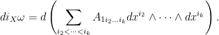
We now recall one more operation, on ${k}$ -forms. If ${\omega}$ is a ${k}$ -form and ${X}$ a vector field, define the interior product

$\displaystyle i_X \omega( A_1, \dots, A_{k-1}) := \omega( A_1, \dots, A_{k-1},X).$

Proposition 3 (Cartan’s magic formula)

We have $\displaystyle L_X = i_X d + d i_X$

on ${k}$ -forms.

Kobayashi-Nomizu prove this using arguments about derivations and skew-derivations, but again it is not necessary. We repeat the same argument, and note that it suffices to treat the case ${X(p) \neq 0}$ . So pick local coordinates ${x^1, \dots, x^n}$ such that ${X = \partial_1}$ . Write

$\displaystyle \omega = \sum_{i_1 < \dots < i_k} A_{i_1 \dots i_k} dx^{i_1} \wedge \dots \wedge dx^{i_k}.$

Then

$\displaystyle di_X \omega = d\left( \sum_{i_2 < \dots < i_k} A_{1 i_2 \dots i_k} dx^{i_2} \wedge \dots \wedge dx^{i_k} \right).$

Also,

$\displaystyle i_X d\omega = \sum_{i_1 < \dots < i_k \\ j} \partial_j A_{i_1\dots i_k} dx^j \wedge dx^{i_1} \wedge \dots \wedge dx^{i_k}$

Adding these gives the result, since

$\displaystyle L_X(\omega) = \sum_{i_1 < \dots < i_k} \partial_1 A_{i_1 \dots i_k} dx^{i_1} \wedge \dots \wedge dx^{i_k} .$

Time-dependent vector fields

A time-dependent vector field ${X}$ is a map from an open subset of ${\mathbb{R} \times M}$ containing ${\{0\} \times M}$ into ${TM}$ such that ${X(t,p) \in T_p(X)}$ . This can be regarded as a generalization of a time-independent vector field. These too generate differential equations: we can talk about an integral curve ${c}$ of a time-dependent vector field as one that satisfies

$\displaystyle \dot{c}(t) = X( t, c(t)).$

This is an ordinary differential equation. In particular, we can locally draw integral curves through a given point, and generate an analog of a “flow” in tthe time-independent case—the difference is that there is no semigroup property ${\phi_{t} \phi_u = \phi_{t+u}}$ .

Conversely:

Proposition 4 Let ${M}$ be a manifold, ${U \subset M}$ an open subset, ${G: I \times U \rightarrow M}$ be an isotopy—that is ${G(t, \cdot)}$ is a diffeomorphism of ${U}$ into ${M}$ . Then ${G}$ corresponds in this manner to a time-dependent vector-field